Harmonic Oscillator

The harmonic oscillator is the most frequently used model in quantum physics.

Definitions

Antique.HarmonicOscillators.HarmonicOscillator — Type

Model

This model is described with the time-independent Schrödinger equation

\[ \hat{H} \psi(x) = E \psi(x),\]

and the Hamiltonian

\[ \hat{H} = - \frac{\hbar^2}{2m} \frac{\mathrm{d}^2}{\mathrm{d}x ^2} + \frac{1}{2} k x^2.\]

Parameters are specified with the following struct:

HO = HarmonicOscillator(k=1.0, m=1.0, hbar=1.0)

$k$ is the force constant, $m$ is the mass of the particle and $\hbar$ is the reduced Planck constant (Dirac's constant).

References

Main:

[3] The Digital Library of Mathematical Functions (DLMF) 18.5.18
[4] C++ Japanese Reference cpprefjp, laguerre_polynomial
[1] D. J. Griffiths, D. F. Schroeter, Introduction to Quantum Mechanics Third Edition (Cambridge University Press, 2018) p.48, 2.3.2 Analytic Method

Supplemental:

[3] The Digital Library of Mathematical Functions (DLMF) 18.3 Table1, 18.5 Table1, 18.5.13, 18.5.18
[5] L. D. Landau, E. M. Lifshitz, Quantum Mechanics (Pergamon Press, 1965) p.595 (a.4), (a.6)
[6] L. I. Schiff, Quantum Mechanics (McGraw-Hill Book Company, 1968) p.71 (13.12)
[7] A. Messiah, Quanfum Mechanics (Dover Publications, 1999) p.491 (B.59)
[8] W. Greiner, Quantum Mechanics: An Introduction Third Edition (Springer, 1994) p.152 (7.22)
[9] D. J. Griffiths, Introduction to Quantum Mechanics (Prentice Hall, 1995) p.41 Table 2.1, p.43 (2.70)
[10] D. A. McQuarrie, J. D. Simon, Physical Chemistry: A Molecular Approach (University Science Books, 1997) p.170 Table 5.2
[11] P. W. Atkins, J. De Paula, Atkins' Physical Chemistry, 8th edition (W. H. Freeman, 2008) p.293 Table 9.1
[12] J. J. Sakurai, J. Napolitano, Modern Quantum Mechanics Third Edition (Cambridge University Press, 2021) p.524 (B.29)

source

Potential

Antique.potential — Method

potential(model::HarmonicOscillator, x)

\[V(x) = \frac{1}{2} k x^2 = \frac{1}{2} m \omega^2 x^2 = \frac{1}{2} \hbar \omega \xi^2,\]

where $\omega = \sqrt{k/m}$ is the angular frequency and $\xi = \sqrt{\frac{m\omega}{\hbar}}x$.

source

Eigenvalues

Antique.energy — Method

energy(model::HarmonicOscillator; n::Integer=0)

\[E_n = \hbar \omega \left( n + \frac{1}{2} \right),\]

where $\omega = \sqrt{k/m}$ is the angular frequency.

source

Eigenfunctions

Antique.wavefunction — Method

wavefunction(model::HarmonicOscillator, x; n::Integer=0)

\[\psi_n(x) = A_n H_n(\xi) \exp{\left( -\frac{\xi^2}{2} \right)},\]

where $\omega = \sqrt{k/m}$, $\xi = \sqrt{\frac{m\omega}{\hbar}}x$, $A_n = \sqrt{\frac{1}{n! 2^n} \sqrt{\frac{m\omega}{\pi\hbar}}}$, $H_n(x) = (-1)^n \mathrm{e}^{x^2} \frac{\mathrm{d}^n}{\mathrm{d}x^n} \mathrm{e}^{-x^2}$ are defined.

source

Hermite Polynomials

Antique.laguerre_polynomial — Method

laguerre_polynomial(model::HarmonicOscillator, x; n=0)

Note

The closed-form expression has been verified to be numerically stable up to $n=10$. For larger $n$, numerical instabilities may arise; a recurrence-relation implementation will address this limitation.

Rodrigues' formula & closed-form:

\[\begin{aligned} H_{n}(x) &:= (-1)^n \mathrm{e}^{x^2} \frac{\mathrm{d}^n}{\mathrm{d}x^n} \mathrm{e}^{-x^2} \\ &= n! \sum_{m=0}^{\lfloor n/2 \rfloor} \frac{(-1)^m}{m! (n-2m)!}(2 x)^{n-2m}. \end{aligned}\]

Examples:

\[\begin{aligned} H_{0}(x) &= 1, \\ H_{1}(x) &= 2 x, \\ H_{2}(x) &= -2 + 4 x^{2}, \\ H_{3}(x) &= -12 x + 8 x^{3}, \\ H_{4}(x) &= 12 - 48 x^{2} + 16 x^{4}, \\ H_{5}(x) &= 120 x - 160 x^{3} + 32 x^{5}, \\ H_{6}(x) &= -120 + 720 x^{2} - 480 x^{4} + 64 x^{6}, \\ H_{7}(x) &= -1680 x + 3360 x^{3} - 1344 x^{5} + 128 x^{7}, \\ H_{8}(x) &= 1680 - 13440 x^{2} + 13440 x^{4} - 3584 x^{6} + 256 x^{8}, \\ H_{9}(x) &= 30240 x - 80640 x^{3} + 48384 x^{5} - 9216 x^{7} + 512 x^{9}, \\ &\vdots \end{aligned}\]

source

Usage & Examples

Install Antique.jl for the first use and run using Antique before each use. The energy energy(), wave function wavefunction() and potential potential() will be exported. In this system, the model is generated by HarmonicOscillator and several parameters k, m and hbar are set as optional arguments.

using Antique
HO = HarmonicOscillator(k=1.0, m=1.0, hbar=1.0)

Parameters:

julia> HO.k1.0
julia> HO.m1.0
julia> HO.hbar1.0

Eigenvalues:

julia> energy(HO, n=0)0.5
julia> energy(HO, n=1)1.5

Potential energy curve:

using CairoMakie

f = Figure()
ax = Axis(f[1,1], xlabel=L"$x$", ylabel=L"$V(x)$")
lines!(ax, -5..5, x -> potential(HO, x))
f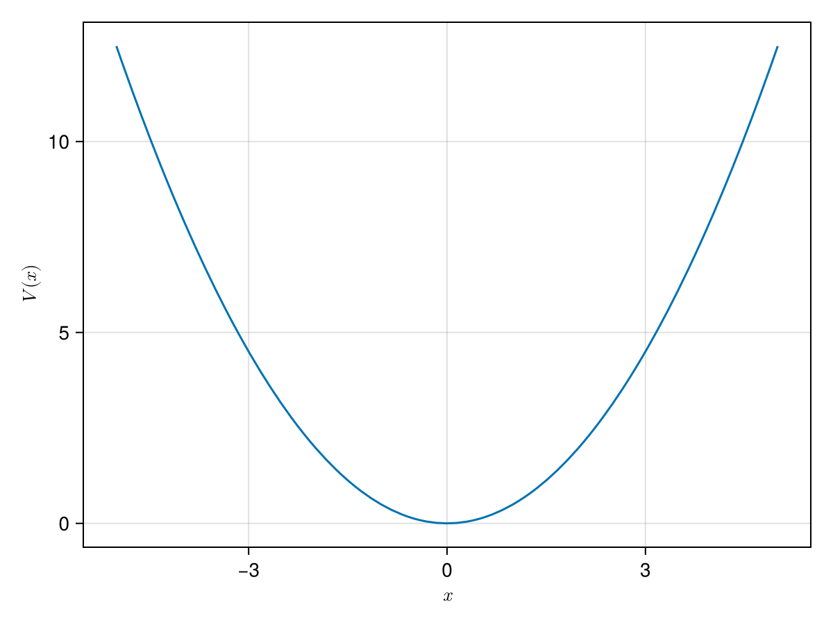

Wave functions:

using CairoMakie

# setting
f = Figure()
ax = Axis(f[1,1], xlabel=L"$x$", ylabel=L"$\psi(x)$")

# plot
w0 = lines!(ax, -5..5, x -> wavefunction(HO, x, n=0))
w1 = lines!(ax, -5..5, x -> wavefunction(HO, x, n=1))
w2 = lines!(ax, -5..5, x -> wavefunction(HO, x, n=2))
w3 = lines!(ax, -5..5, x -> wavefunction(HO, x, n=3))
w4 = lines!(ax, -5..5, x -> wavefunction(HO, x, n=4))

# legend
axislegend(ax, [w0, w1, w2, w3, w4], [L"n=0", L"n=1", L"n=2", L"n=3", L"n=4"], position=:lb)

f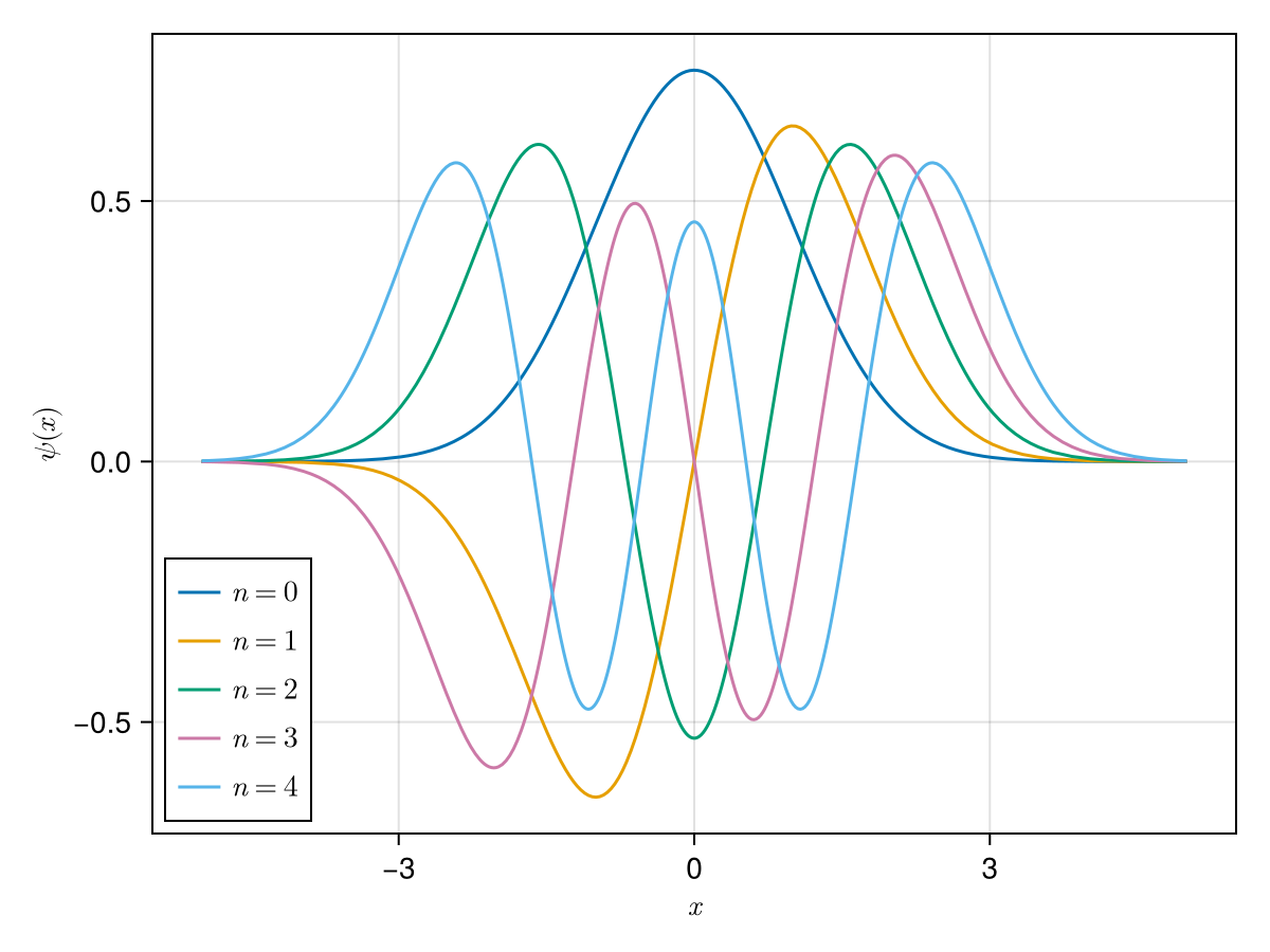

Potential energy curve, Energy levels, Wave functions:

using CairoMakie

# settings
f = Figure()
ax = Axis(f[1,1], xlabel=L"$x$", ylabel=L"$V(x),~E_n,~\psi_n(x) \times 5 + E_n$", aspect=1, limits=(-5,5,0,5.2))
# hidespines!(ax)
# hidedecorations!(ax)

for n in 0:4
  # classical turning point
  xE = sqrt(2*HO.k*energy(HO, n=n))
  # energy
  lines!(ax, [-xE,xE], fill(energy(HO,n=n),2), color=:black, linewidth=2)
  hlines!(ax, energy(HO, n=n), color=:black, linewidth=1, linestyle=:dash)
  # wave function
  lines!(ax, -5..5, x -> energy(HO,n=n) + 0.5*wavefunction(HO,x,n=n), linewidth=2)
end

#potential
lines!(ax, -5..5, x -> potential(HO, x), color=:black, linewidth=2)

f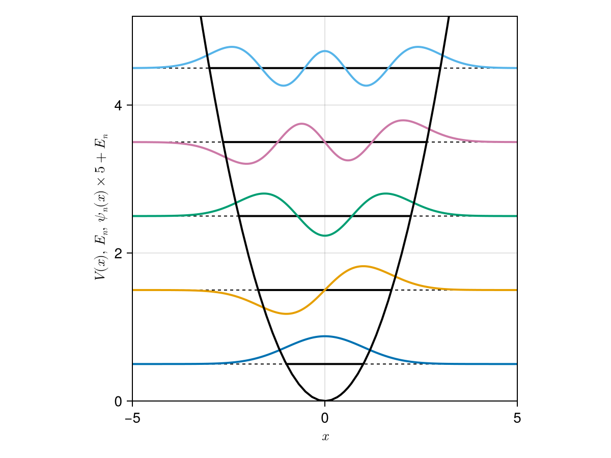

Testing

Unit testing and Integration testing were done using a computer algebra system (Symbolics.jl) and numerical integration (QuadGK.jl). The test script is here.

Hermite Polynomials $H_n(x)$

\[ \begin{aligned} H_{n}(x) &:= (-1)^n \mathrm{e}^{x^2} \frac{\mathrm{d}^n}{\mathrm{d}x^n} \mathrm{e}^{-x^2} \\ &= n! \sum_{m=0}^{\lfloor n/2 \rfloor} \frac{(-1)^m}{m! (n-2m)!}(2 x)^{n-2m}. \end{aligned}\]

$n=0:$ ✔

\[\begin{aligned} H_{0}(x) = e^{ - x^{2}} e^{x^{2}} &= 1 \\ &= 1 \end{aligned}\]

$n=1:$ ✔

\[\begin{aligned} H_{1}(x) = - e^{x^{2}} \frac{\mathrm{d} e^{ - x^{2}}}{\mathrm{d}x} &= 2 x \\ &= 2 x \end{aligned}\]

$n=2:$ ✔

\[\begin{aligned} H_{2}(x) = e^{x^{2}} \frac{\mathrm{d}}{\mathrm{d}x} \frac{\mathrm{d} e^{ - x^{2}}}{\mathrm{d}x} &= -2 + 4 x^{2} \\ &= -2 + 4 x^{2} \end{aligned}\]

$n=3:$ ✔

\[\begin{aligned} H_{3}(x) = - e^{x^{2}} \frac{\mathrm{d}}{\mathrm{d}x} \frac{\mathrm{d}}{\mathrm{d}x} \frac{\mathrm{d} e^{ - x^{2}}}{\mathrm{d}x} &= - 12 x + 8 x^{3} \\ &= - 12 x + 8 x^{3} \end{aligned}\]

$n=4:$ ✔

\[\begin{aligned} H_{4}(x) = e^{x^{2}} \frac{\mathrm{d}}{\mathrm{d}x} \frac{\mathrm{d}}{\mathrm{d}x} \frac{\mathrm{d}}{\mathrm{d}x} \frac{\mathrm{d} e^{ - x^{2}}}{\mathrm{d}x} &= 12 - 48 x^{2} + 16 x^{4} \\ &= 12 - 48 x^{2} + 16 x^{4} \end{aligned}\]

$n=5:$ ✔

\[\begin{aligned} H_{5}(x) = - \frac{\mathrm{d}}{\mathrm{d}x} \frac{\mathrm{d}}{\mathrm{d}x} \frac{\mathrm{d}}{\mathrm{d}x} \frac{\mathrm{d}}{\mathrm{d}x} \frac{\mathrm{d} e^{ - x^{2}}}{\mathrm{d}x} e^{x^{2}} &= 120 x - 160 x^{3} + 32 x^{5} \\ &= 120 x - 160 x^{3} + 32 x^{5} \end{aligned}\]

$n=6:$ ✔

\[\begin{aligned} H_{6}(x) = e^{x^{2}} \frac{\mathrm{d}}{\mathrm{d}x} \frac{\mathrm{d}}{\mathrm{d}x} \frac{\mathrm{d}}{\mathrm{d}x} \frac{\mathrm{d}}{\mathrm{d}x} \frac{\mathrm{d}}{\mathrm{d}x} \frac{\mathrm{d} e^{ - x^{2}}}{\mathrm{d}x} &= -120 + 720 x^{2} - 480 x^{4} + 64 x^{6} \\ &= -120 + 720 x^{2} - 480 x^{4} + 64 x^{6} \end{aligned}\]

$n=7:$ ✔

\[\begin{aligned} H_{7}(x) = - e^{x^{2}} \frac{\mathrm{d}}{\mathrm{d}x} \frac{\mathrm{d}}{\mathrm{d}x} \frac{\mathrm{d}}{\mathrm{d}x} \frac{\mathrm{d}}{\mathrm{d}x} \frac{\mathrm{d}}{\mathrm{d}x} \frac{\mathrm{d}}{\mathrm{d}x} \frac{\mathrm{d} e^{ - x^{2}}}{\mathrm{d}x} &= - 1680 x + 3360 x^{3} - 1344 x^{5} + 128 x^{7} \\ &= - 1680 x + 3360 x^{3} - 1344 x^{5} + 128 x^{7} \end{aligned}\]

$n=8:$ ✔

\[\begin{aligned} H_{8}(x) = e^{x^{2}} \frac{\mathrm{d}}{\mathrm{d}x} \frac{\mathrm{d}}{\mathrm{d}x} \frac{\mathrm{d}}{\mathrm{d}x} \frac{\mathrm{d}}{\mathrm{d}x} \frac{\mathrm{d}}{\mathrm{d}x} \frac{\mathrm{d}}{\mathrm{d}x} \frac{\mathrm{d}}{\mathrm{d}x} \frac{\mathrm{d} e^{ - x^{2}}}{\mathrm{d}x} &= 1680 - 13440 x^{2} + 13440 x^{4} - 3584 x^{6} + 256 x^{8} \\ &= 1680 - 13440 x^{2} + 13440 x^{4} - 3584 x^{6} + 256 x^{8} \end{aligned}\]

$n=9:$ ✔

\[\begin{aligned} H_{9}(x) = - e^{x^{2}} \frac{\mathrm{d}}{\mathrm{d}x} \frac{\mathrm{d}}{\mathrm{d}x} \frac{\mathrm{d}}{\mathrm{d}x} \frac{\mathrm{d}}{\mathrm{d}x} \frac{\mathrm{d}}{\mathrm{d}x} \frac{\mathrm{d}}{\mathrm{d}x} \frac{\mathrm{d}}{\mathrm{d}x} \frac{\mathrm{d}}{\mathrm{d}x} \frac{\mathrm{d} e^{ - x^{2}}}{\mathrm{d}x} &= 30240 x - 80640 x^{3} + 48384 x^{5} - 9216 x^{7} + 512 x^{9} \\ &= 30240 x - 80640 x^{3} + 48384 x^{5} - 9216 x^{7} + 512 x^{9} \end{aligned}\]

Normalization & Orthogonality of $H_n(x)$

\[\int_{-\infty}^\infty H_j(x) H_i(x) \mathrm{e}^{-x^2} \mathrm{d}x = \sqrt{\pi} 2^j j! \delta_{ij}\]

 i |  j |     analytical |      numerical 
-- | -- | -------------- | -------------- 
 0 |  0 |    1.772453851 |    1.772453851 ✔
 0 |  1 |    0.000000000 |    0.000000000 ✔
 0 |  2 |    0.000000000 |    0.000000000 ✔
 0 |  3 |    0.000000000 |    0.000000000 ✔
 0 |  4 |    0.000000000 |   -0.000000000 ✔
 0 |  5 |    0.000000000 |   -0.000000000 ✔
 0 |  6 |    0.000000000 |    0.000000000 ✔
 0 |  7 |    0.000000000 |    0.000000000 ✔
 0 |  8 |    0.000000000 |   -0.000000000 ✔
 0 |  9 |    0.000000000 |    0.000000000 ✔
 1 |  0 |    0.000000000 |    0.000000000 ✔
 1 |  1 |    3.544907702 |    3.544907702 ✔
 1 |  2 |    0.000000000 |    0.000000000 ✔
 1 |  3 |    0.000000000 |   -0.000000000 ✔
 1 |  4 |    0.000000000 |   -0.000000000 ✔
 1 |  5 |    0.000000000 |    0.000000000 ✔
 1 |  6 |    0.000000000 |    0.000000000 ✔
 1 |  7 |    0.000000000 |   -0.000000000 ✔
 1 |  8 |    0.000000000 |   -0.000000000 ✔
 1 |  9 |    0.000000000 |    0.000000000 ✔
 2 |  0 |    0.000000000 |    0.000000000 ✔
 2 |  1 |    0.000000000 |    0.000000000 ✔
 2 |  2 |   14.179630807 |   14.179630807 ✔
 2 |  3 |    0.000000000 |   -0.000000000 ✔
 2 |  4 |    0.000000000 |   -0.000000000 ✔
 2 |  5 |    0.000000000 |    0.000000000 ✔
 2 |  6 |    0.000000000 |    0.000000000 ✔
 2 |  7 |    0.000000000 |   -0.000000000 ✔
 2 |  8 |    0.000000000 |   -0.000000000 ✔
 2 |  9 |    0.000000000 |   -0.000000000 ✔
 3 |  0 |    0.000000000 |    0.000000000 ✔
 3 |  1 |    0.000000000 |   -0.000000000 ✔
 3 |  2 |    0.000000000 |   -0.000000000 ✔
 3 |  3 |   85.077784843 |   85.077784843 ✔
 3 |  4 |    0.000000000 |   -0.000000000 ✔
 3 |  5 |    0.000000000 |    0.000000000 ✔
 3 |  6 |    0.000000000 |   -0.000000000 ✔
 3 |  7 |    0.000000000 |   -0.000000000 ✔
 3 |  8 |    0.000000000 |   -0.000000000 ✔
 3 |  9 |    0.000000000 |    0.000000000 ✔
 4 |  0 |    0.000000000 |   -0.000000000 ✔
 4 |  1 |    0.000000000 |   -0.000000000 ✔
 4 |  2 |    0.000000000 |   -0.000000000 ✔
 4 |  3 |    0.000000000 |   -0.000000000 ✔
 4 |  4 |  680.622278748 |  680.622278748 ✔
 4 |  5 |    0.000000000 |    0.000000000 ✔
 4 |  6 |    0.000000000 |    0.000000000 ✔
 4 |  7 |    0.000000000 |    0.000000000 ✔
 4 |  8 |    0.000000000 |   -0.000000000 ✔
 4 |  9 |    0.000000000 |   -0.000000000 ✔
 5 |  0 |    0.000000000 |   -0.000000000 ✔
 5 |  1 |    0.000000000 |    0.000000000 ✔
 5 |  2 |    0.000000000 |    0.000000000 ✔
 5 |  3 |    0.000000000 |    0.000000000 ✔
 5 |  4 |    0.000000000 |    0.000000000 ✔
 5 |  5 | 6806.222787477 | 6806.222787477 ✔
 5 |  6 |    0.000000000 |    0.000000000 ✔
 5 |  7 |    0.000000000 |    0.000000000 ✔
 5 |  8 |    0.000000000 |    0.000000000 ✔
 5 |  9 |    0.000000000 |    0.000000001 ✔
 6 |  0 |    0.000000000 |    0.000000000 ✔
 6 |  1 |    0.000000000 |    0.000000000 ✔
 6 |  2 |    0.000000000 |    0.000000000 ✔
 6 |  3 |    0.000000000 |   -0.000000000 ✔
 6 |  4 |    0.000000000 |    0.000000000 ✔
 6 |  5 |    0.000000000 |    0.000000000 ✔
 6 |  6 | 81674.673449726 | 81674.673449726 ✔
 6 |  7 |    0.000000000 |    0.000000000 ✔
 6 |  8 |    0.000000000 |    0.000000000 ✔
 6 |  9 |    0.000000000 |   -0.000000000 ✔
 7 |  0 |    0.000000000 |    0.000000000 ✔
 7 |  1 |    0.000000000 |   -0.000000000 ✔
 7 |  2 |    0.000000000 |   -0.000000000 ✔
 7 |  3 |    0.000000000 |   -0.000000000 ✔
 7 |  4 |    0.000000000 |    0.000000000 ✔
 7 |  5 |    0.000000000 |    0.000000000 ✔
 7 |  6 |    0.000000000 |    0.000000000 ✔
 7 |  7 | 1143445.428296166 | 1143445.428296166 ✔
 7 |  8 |    0.000000000 |   -0.000000000 ✔
 7 |  9 |    0.000000000 |    0.000000007 ✔
 8 |  0 |    0.000000000 |   -0.000000000 ✔
 8 |  1 |    0.000000000 |   -0.000000000 ✔
 8 |  2 |    0.000000000 |   -0.000000000 ✔
 8 |  3 |    0.000000000 |   -0.000000000 ✔
 8 |  4 |    0.000000000 |   -0.000000000 ✔
 8 |  5 |    0.000000000 |    0.000000000 ✔
 8 |  6 |    0.000000000 |    0.000000000 ✔
 8 |  7 |    0.000000000 |   -0.000000000 ✔
 8 |  8 | 18295126.852738664 | 18295126.852738667 ✔
 8 |  9 |    0.000000000 |    0.000000001 ✔
 9 |  0 |    0.000000000 |    0.000000000 ✔
 9 |  1 |    0.000000000 |    0.000000000 ✔
 9 |  2 |    0.000000000 |   -0.000000000 ✔
 9 |  3 |    0.000000000 |    0.000000000 ✔
 9 |  4 |    0.000000000 |   -0.000000000 ✔
 9 |  5 |    0.000000000 |    0.000000001 ✔
 9 |  6 |    0.000000000 |   -0.000000000 ✔
 9 |  7 |    0.000000000 |    0.000000007 ✔
 9 |  8 |    0.000000000 |    0.000000001 ✔
 9 |  9 | 329312283.349295914 | 329312283.349295735 ✔

Normalization & Orthogonality of $\psi_n(x)$

\[\int \psi_i^\ast(x) \psi_j(x) \mathrm{d}x = \delta_{ij}\]

 i |  j |     analytical |      numerical 
-- | -- | -------------- | -------------- 
 0 |  0 |    1.000000000 |    1.000000000 ✔
 0 |  1 |    0.000000000 |    0.000000000 ✔
 0 |  2 |    0.000000000 |    0.000000000 ✔
 0 |  3 |    0.000000000 |    0.000000000 ✔
 0 |  4 |    0.000000000 |   -0.000000000 ✔
 0 |  5 |    0.000000000 |    0.000000000 ✔
 0 |  6 |    0.000000000 |    0.000000000 ✔
 0 |  7 |    0.000000000 |   -0.000000000 ✔
 0 |  8 |    0.000000000 |   -0.000000000 ✔
 0 |  9 |    0.000000000 |    0.000000000 ✔
 1 |  0 |    0.000000000 |    0.000000000 ✔
 1 |  1 |    1.000000000 |    1.000000000 ✔
 1 |  2 |    0.000000000 |    0.000000000 ✔
 1 |  3 |    0.000000000 |   -0.000000000 ✔
 1 |  4 |    0.000000000 |   -0.000000000 ✔
 1 |  5 |    0.000000000 |    0.000000000 ✔
 1 |  6 |    0.000000000 |   -0.000000000 ✔
 1 |  7 |    0.000000000 |   -0.000000000 ✔
 1 |  8 |    0.000000000 |    0.000000000 ✔
 1 |  9 |    0.000000000 |    0.000000000 ✔
 2 |  0 |    0.000000000 |    0.000000000 ✔
 2 |  1 |    0.000000000 |    0.000000000 ✔
 2 |  2 |    1.000000000 |    1.000000000 ✔
 2 |  3 |    0.000000000 |   -0.000000000 ✔
 2 |  4 |    0.000000000 |   -0.000000000 ✔
 2 |  5 |    0.000000000 |    0.000000000 ✔
 2 |  6 |    0.000000000 |    0.000000000 ✔
 2 |  7 |    0.000000000 |   -0.000000000 ✔
 2 |  8 |    0.000000000 |   -0.000000000 ✔
 2 |  9 |    0.000000000 |    0.000000000 ✔
 3 |  0 |    0.000000000 |    0.000000000 ✔
 3 |  1 |    0.000000000 |   -0.000000000 ✔
 3 |  2 |    0.000000000 |   -0.000000000 ✔
 3 |  3 |    1.000000000 |    1.000000000 ✔
 3 |  4 |    0.000000000 |   -0.000000000 ✔
 3 |  5 |    0.000000000 |    0.000000000 ✔
 3 |  6 |    0.000000000 |    0.000000000 ✔
 3 |  7 |    0.000000000 |   -0.000000000 ✔
 3 |  8 |    0.000000000 |   -0.000000000 ✔
 3 |  9 |    0.000000000 |    0.000000000 ✔
 4 |  0 |    0.000000000 |   -0.000000000 ✔
 4 |  1 |    0.000000000 |   -0.000000000 ✔
 4 |  2 |    0.000000000 |   -0.000000000 ✔
 4 |  3 |    0.000000000 |   -0.000000000 ✔
 4 |  4 |    1.000000000 |    1.000000000 ✔
 4 |  5 |    0.000000000 |   -0.000000000 ✔
 4 |  6 |    0.000000000 |    0.000000000 ✔
 4 |  7 |    0.000000000 |    0.000000000 ✔
 4 |  8 |    0.000000000 |   -0.000000000 ✔
 4 |  9 |    0.000000000 |   -0.000000000 ✔
 5 |  0 |    0.000000000 |    0.000000000 ✔
 5 |  1 |    0.000000000 |    0.000000000 ✔
 5 |  2 |    0.000000000 |    0.000000000 ✔
 5 |  3 |    0.000000000 |    0.000000000 ✔
 5 |  4 |    0.000000000 |   -0.000000000 ✔
 5 |  5 |    1.000000000 |    1.000000000 ✔
 5 |  6 |    0.000000000 |    0.000000000 ✔
 5 |  7 |    0.000000000 |    0.000000000 ✔
 5 |  8 |    0.000000000 |    0.000000000 ✔
 5 |  9 |    0.000000000 |    0.000000000 ✔
 6 |  0 |    0.000000000 |    0.000000000 ✔
 6 |  1 |    0.000000000 |   -0.000000000 ✔
 6 |  2 |    0.000000000 |    0.000000000 ✔
 6 |  3 |    0.000000000 |    0.000000000 ✔
 6 |  4 |    0.000000000 |    0.000000000 ✔
 6 |  5 |    0.000000000 |    0.000000000 ✔
 6 |  6 |    1.000000000 |    1.000000000 ✔
 6 |  7 |    0.000000000 |    0.000000000 ✔
 6 |  8 |    0.000000000 |    0.000000000 ✔
 6 |  9 |    0.000000000 |    0.000000000 ✔
 7 |  0 |    0.000000000 |   -0.000000000 ✔
 7 |  1 |    0.000000000 |   -0.000000000 ✔
 7 |  2 |    0.000000000 |   -0.000000000 ✔
 7 |  3 |    0.000000000 |   -0.000000000 ✔
 7 |  4 |    0.000000000 |    0.000000000 ✔
 7 |  5 |    0.000000000 |    0.000000000 ✔
 7 |  6 |    0.000000000 |    0.000000000 ✔
 7 |  7 |    1.000000000 |    1.000000000 ✔
 7 |  8 |    0.000000000 |    0.000000000 ✔
 7 |  9 |    0.000000000 |    0.000000000 ✔
 8 |  0 |    0.000000000 |   -0.000000000 ✔
 8 |  1 |    0.000000000 |    0.000000000 ✔
 8 |  2 |    0.000000000 |   -0.000000000 ✔
 8 |  3 |    0.000000000 |   -0.000000000 ✔
 8 |  4 |    0.000000000 |   -0.000000000 ✔
 8 |  5 |    0.000000000 |    0.000000000 ✔
 8 |  6 |    0.000000000 |    0.000000000 ✔
 8 |  7 |    0.000000000 |    0.000000000 ✔
 8 |  8 |    1.000000000 |    1.000000000 ✔
 8 |  9 |    0.000000000 |   -0.000000000 ✔
 9 |  0 |    0.000000000 |    0.000000000 ✔
 9 |  1 |    0.000000000 |    0.000000000 ✔
 9 |  2 |    0.000000000 |    0.000000000 ✔
 9 |  3 |    0.000000000 |    0.000000000 ✔
 9 |  4 |    0.000000000 |   -0.000000000 ✔
 9 |  5 |    0.000000000 |    0.000000000 ✔
 9 |  6 |    0.000000000 |    0.000000000 ✔
 9 |  7 |    0.000000000 |    0.000000000 ✔
 9 |  8 |    0.000000000 |   -0.000000000 ✔
 9 |  9 |    1.000000000 |    1.000000000 ✔

Virial Theorem

The virial theorem $\langle T \rangle = \langle V \rangle$ and the definition of Hamiltonian $\langle H \rangle = \langle T \rangle + \langle V \rangle$ derive $\langle H \rangle = 2 \langle V \rangle = 2 \langle T \rangle$.

\[2 \int \psi_n^\ast(x) potential(x) \psi_n(x) \mathrm{d}x = E_n\]

  k |  n |     analytical |      numerical 
--- | -- | -------------- | -------------- 
0.1 |  0 |    0.500000000 |    0.500000000 ✔
0.1 |  1 |    1.500000000 |    1.500000000 ✔
0.1 |  2 |    2.500000000 |    2.500000000 ✔
0.1 |  3 |    3.500000000 |    3.500000000 ✔
0.1 |  4 |    4.500000000 |    4.500000000 ✔
0.1 |  5 |    5.500000000 |    5.500000000 ✔
0.1 |  6 |    6.500000000 |    6.500000000 ✔
0.1 |  7 |    7.500000000 |    7.500000000 ✔
0.1 |  8 |    8.500000000 |    8.500000000 ✔
0.1 |  9 |    9.500000000 |    9.500000000 ✔
0.5 |  0 |    0.500000000 |    0.500000000 ✔
0.5 |  1 |    1.500000000 |    1.500000000 ✔
0.5 |  2 |    2.500000000 |    2.500000000 ✔
0.5 |  3 |    3.500000000 |    3.500000000 ✔
0.5 |  4 |    4.500000000 |    4.500000000 ✔
0.5 |  5 |    5.500000000 |    5.500000000 ✔
0.5 |  6 |    6.500000000 |    6.500000000 ✔
0.5 |  7 |    7.500000000 |    7.500000000 ✔
0.5 |  8 |    8.500000000 |    8.500000000 ✔
0.5 |  9 |    9.500000000 |    9.500000000 ✔
1.0 |  0 |    0.500000000 |    0.500000000 ✔
1.0 |  1 |    1.500000000 |    1.500000000 ✔
1.0 |  2 |    2.500000000 |    2.500000000 ✔
1.0 |  3 |    3.500000000 |    3.500000000 ✔
1.0 |  4 |    4.500000000 |    4.500000000 ✔
1.0 |  5 |    5.500000000 |    5.500000000 ✔
1.0 |  6 |    6.500000000 |    6.500000000 ✔
1.0 |  7 |    7.500000000 |    7.500000000 ✔
1.0 |  8 |    8.500000000 |    8.500000000 ✔
1.0 |  9 |    9.500000000 |    9.500000000 ✔
5.0 |  0 |    0.500000000 |    0.500000000 ✔
5.0 |  1 |    1.500000000 |    1.500000000 ✔
5.0 |  2 |    2.500000000 |    2.500000000 ✔
5.0 |  3 |    3.500000000 |    3.500000000 ✔
5.0 |  4 |    4.500000000 |    4.500000000 ✔
5.0 |  5 |    5.500000000 |    5.500000000 ✔
5.0 |  6 |    6.500000000 |    6.500000000 ✔
5.0 |  7 |    7.500000000 |    7.500000000 ✔
5.0 |  8 |    8.500000000 |    8.500000000 ✔
5.0 |  9 |    9.500000000 |    9.500000000 ✔

Eigenvalues

\[ \begin{aligned} E_n &= \int \psi^\ast_n(x) \hat{H} \psi_n(x) \mathrm{d}x \\ &= \int \psi^\ast_n(x) \left[ \hat{V} + \hat{T} \right] \psi(x) \mathrm{d}x \\ &= \int \psi^\ast_n(x) \left[ potential(x) - \frac{\hbar^2}{2m} \frac{\mathrm{d}^{2}}{\mathrm{d} x^{2}} \right] \psi(x) \mathrm{d}x \\ &\simeq \int \psi^\ast_n(x) \left[ potential(x)\psi(x) -\frac{\hbar^2}{2m} \frac{\psi(x+\Delta x) - 2\psi(x) + \psi(x-\Delta x)}{\Delta x^{2}} \right] \mathrm{d}x. \end{aligned}\]

Where, the difference formula for the 2nd-order derivative:

\[\begin{aligned} % 2\psi(x) % + \frac{\mathrm{d}^{2} \psi(x)}{\mathrm{d} x^{2}} \Delta x^{2} % + O\left(\Delta x^{4}\right) % &= % \psi(x+\Delta x) % + \psi(x-\Delta x) % \\ % \frac{\mathrm{d}^{2} \psi(x)}{\mathrm{d} x^{2}} \Delta x^{2} % &= % \psi(x+\Delta x) % - 2\psi(x) % + \psi(x-\Delta x) % - O\left(\Delta x^{4}\right) % \\ % \frac{\mathrm{d}^{2} \psi(x)}{\mathrm{d} x^{2}} % &= % \frac{\psi(x+\Delta x) - 2\psi(x) + \psi(x-\Delta x)}{\Delta x^{2}} % - \frac{O\left(\Delta x^{4}\right)}{\Delta x^{2}} % \\ \frac{\mathrm{d}^{2} \psi(x)}{\mathrm{d} x^{2}} &= \frac{\psi(x+\Delta x) - 2\psi(x) + \psi(x-\Delta x)}{\Delta x^{2}} + O\left(\Delta x^{2}\right) \end{aligned}\]

are given by the sum of 2 Taylor series:

\[\begin{aligned} \psi(x+\Delta x) &= \psi(x) + \frac{\mathrm{d} \psi(x)}{\mathrm{d} x} \Delta x + \frac{1}{2!} \frac{\mathrm{d}^{2} \psi(x)}{\mathrm{d} x^{2}} \Delta x^{2} + \frac{1}{3!} \frac{\mathrm{d}^{3} \psi(x)}{\mathrm{d} x^{3}} \Delta x^{3} + O\left(\Delta x^{4}\right), \\ \psi(x-\Delta x) &= \psi(x) - \frac{\mathrm{d} \psi(x)}{\mathrm{d} x} \Delta x + \frac{1}{2!} \frac{\mathrm{d}^{2} \psi(x)}{\mathrm{d} x^{2}} \Delta x^{2} - \frac{1}{3!} \frac{\mathrm{d}^{3} \psi(x)}{\mathrm{d} x^{3}} \Delta x^{3} + O\left(\Delta x^{4}\right). \end{aligned}\]

  k |  n |     analytical |      numerical 
--- | -- | -------------- | -------------- 
0.1 |  0 |    0.158113883 |    0.158113880 ✔
0.1 |  1 |    0.474341649 |    0.474341633 ✔
0.1 |  2 |    0.790569415 |    0.790569374 ✔
0.1 |  3 |    1.106797181 |    1.106797103 ✔
0.1 |  4 |    1.423024947 |    1.423024819 ✔
0.1 |  5 |    1.739252713 |    1.739252523 ✔
0.1 |  6 |    2.055480479 |    2.055480214 ✔
0.1 |  7 |    2.371708245 |    2.371707892 ✔
0.1 |  8 |    2.687936011 |    2.687935558 ✔
0.1 |  9 |    3.004163777 |    3.004163211 ✔
0.5 |  0 |    0.353553391 |    0.353553375 ✔
0.5 |  1 |    1.060660172 |    1.060660094 ✔
0.5 |  2 |    1.767766953 |    1.767766750 ✔
0.5 |  3 |    2.474873734 |    2.474873344 ✔
0.5 |  4 |    3.181980515 |    3.181979875 ✔
0.5 |  5 |    3.889087297 |    3.889086343 ✔
0.5 |  6 |    4.596194078 |    4.596192750 ✔
0.5 |  7 |    5.303300859 |    5.303299093 ✔
0.5 |  8 |    6.010407640 |    6.010405375 ✔
0.5 |  9 |    6.717514421 |    6.717511593 ✔
1.0 |  0 |    0.500000000 |    0.499999969 ✔
1.0 |  1 |    1.500000000 |    1.499999844 ✔
1.0 |  2 |    2.500000000 |    2.499999594 ✔
1.0 |  3 |    3.500000000 |    3.499999219 ✔
1.0 |  4 |    4.500000000 |    4.499998719 ✔
1.0 |  5 |    5.500000000 |    5.499998094 ✔
1.0 |  6 |    6.500000000 |    6.499997344 ✔
1.0 |  7 |    7.500000000 |    7.499996469 ✔
1.0 |  8 |    8.500000000 |    8.499995469 ✔
1.0 |  9 |    9.500000000 |    9.499994343 ✔
5.0 |  0 |    1.118033989 |    1.118033833 ✔
5.0 |  1 |    3.354101966 |    3.354101185 ✔
5.0 |  2 |    5.590169944 |    5.590167913 ✔
5.0 |  3 |    7.826237921 |    7.826234015 ✔
5.0 |  4 |   10.062305899 |   10.062299492 ✔
5.0 |  5 |   12.298373876 |   12.298364345 ✔
5.0 |  6 |   14.534441854 |   14.534428572 ✔
5.0 |  7 |   16.770509831 |   16.770492175 ✔
5.0 |  8 |   19.006577809 |   19.006555152 ✔
5.0 |  9 |   21.242645786 |   21.242617505 ✔