Delta Potential
The Delta potential is one of the simplest models for a quantum mechanical system in 1D. It always has one bound state and its wave function has a cusp at the origin.
Definitions
Antique.DeltaPotential — Type
Model
This model is described with the time-independent Schrödinger equation
\[ \hat{H} \psi(x) = E \psi(x),\]
and the Hamiltonian
\[ \hat{H} = - \frac{\hbar^2}{2m} \frac{\mathrm{d}^2}{\mathrm{d}x ^2} - \alpha \delta(x).\]
Parameters are specified with the following struct:
DP = DeltaPotential(α=1.0, m=1.0, ℏ=1.0)$\alpha$ is the potential strength, $m$ is the mass of particle and $\hbar$ is the reduced Planck constant (Dirac's constant).
References
- [1] D. J. Griffiths, D. F. Schroeter, Introduction to Quantum Mechanics Third Edition (Cambridge University Press, 2018), (https://doi.org/10.1017/9781316995433) p.63, 2.5.2 The Delta-Function Well
- [2] UCSD Physics 130, Quantum Physics, (https://quantummechanics.ucsd.edu/ph130a/130_notes/node154.html)
Potential
Eigenvalues
Eigenfunctions
Usage & Examples
Install Antique.jl for the first use and run using Antique before each use. The energy E(), wave function ψ() and potential V() will be exported. In this system, the model is generated by DeltaPotential and several parameters α, m and ℏ are set as optional arguments.
using Antique
DP = DeltaPotential(α=1.0, m=1.0, ℏ=1.0)
Parameters:
julia> DP.α1.0julia> DP.m1.0julia> DP.ℏ1.0
Eigenvalues:
julia> E(DP)-0.5
Wave functions:
using CairoMakie

# setting
f = Figure()
ax = Axis(f[1,1], xlabel=L"$x$", ylabel=L"$\psi(x)$")

# plot
w = lines!(ax, -5..5, x -> ψ(DP, x))

f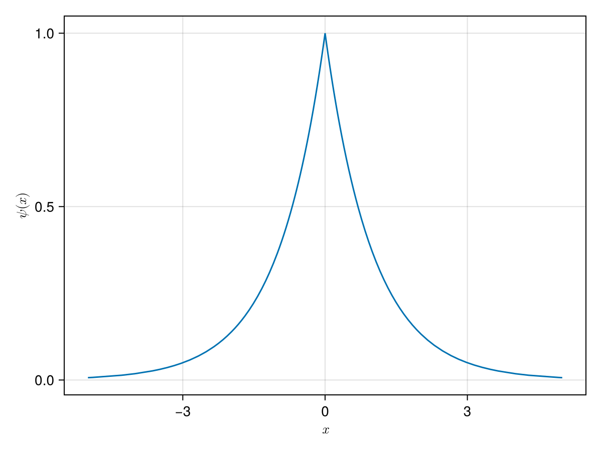
Potential energy curve, energy levels, wave functions:
using CairoMakie

# settings
f = Figure()
ax = Axis(f[1,1], xlabel=L"$x$", ylabel=L"$V(x),~E_n,~\psi_n(x) \times 5 + E_n$", aspect=1, limits=(-5,5,-0.6,0.6))
# hidespines!(ax)
# hidedecorations!(ax)

# energy
hlines!(ax, E(DP), color=:black, linewidth=1, linestyle=:dash)

# wave function
lines!(ax, -5..5, x -> E(DP) + ψ(DP,x), linewidth=2)

#potential
lines!(ax, [-5,0,0,0,5], [0,0,-1,0,0], color=:black, linewidth=2)

f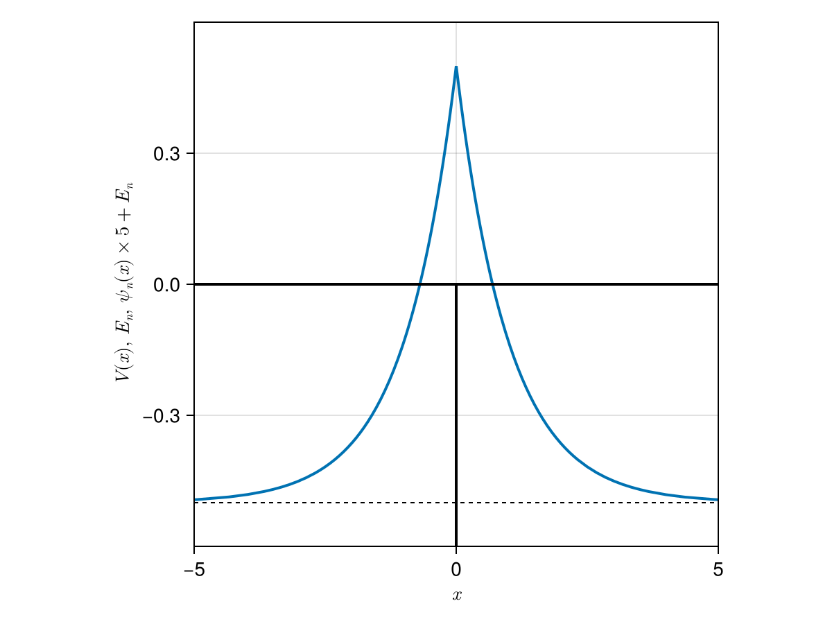
Testing
Unit testing and integration testing were done using numerical integration (QuadGK.jl). The test script is here.
Normalization of $\psi(x)$
\[\int_{-\infty}^{\infty} \psi^\ast(x) \psi(x) ~\mathrm{d}x = 1\]
  α |   m |   ℏ |     analytical |      numerical
--- | --- | --- | -------------- | --------------
0.1 | 0.1 | 0.1 |    1.000000000 |    1.000000000 ✔
0.1 | 0.1 | 1.0 |    1.000000000 |    1.000000000 ✔
0.1 | 0.1 | 7.0 |    1.000000000 |    1.000004676 ✔
0.1 | 1.0 | 0.1 |    1.000000000 |    1.000000000 ✔
0.1 | 1.0 | 1.0 |    1.000000000 |    1.000000000 ✔
0.1 | 1.0 | 7.0 |    1.000000000 |    1.000000000 ✔
0.1 | 7.0 | 0.1 |    1.000000000 |    1.000000000 ✔
0.1 | 7.0 | 1.0 |    1.000000000 |    1.000000000 ✔
0.1 | 7.0 | 7.0 |    1.000000000 |    1.000000000 ✔
1.0 | 0.1 | 0.1 |    1.000000000 |    1.000000000 ✔
1.0 | 0.1 | 1.0 |    1.000000000 |    1.000000000 ✔
1.0 | 0.1 | 7.0 |    1.000000000 |    1.000000000 ✔
1.0 | 1.0 | 0.1 |    1.000000000 |    1.000000000 ✔
1.0 | 1.0 | 1.0 |    1.000000000 |    1.000000000 ✔
1.0 | 1.0 | 7.0 |    1.000000000 |    1.000000000 ✔
1.0 | 7.0 | 0.1 |    1.000000000 |    1.000000000 ✔
1.0 | 7.0 | 1.0 |    1.000000000 |    1.000000000 ✔
1.0 | 7.0 | 7.0 |    1.000000000 |    1.000000000 ✔
7.0 | 0.1 | 0.1 |    1.000000000 |    1.000000000 ✔
7.0 | 0.1 | 1.0 |    1.000000000 |    1.000000000 ✔
7.0 | 0.1 | 7.0 |    1.000000000 |    1.000000000 ✔
7.0 | 1.0 | 0.1 |    1.000000000 |    1.000000000 ✔
7.0 | 1.0 | 1.0 |    1.000000000 |    1.000000000 ✔
7.0 | 1.0 | 7.0 |    1.000000000 |    1.000000000 ✔
7.0 | 7.0 | 0.1 |    1.000000000 |    1.000000000 ✔
7.0 | 7.0 | 1.0 |    1.000000000 |    1.000000000 ✔
7.0 | 7.0 | 7.0 |    1.000000000 |    1.000000000 ✔
Eigenvalues
\[\begin{aligned} E_n &= \int_{-\infty}^{\infty} \psi^\ast(x) \hat{H} \psi(x) ~\mathrm{d}x \\ &= \int_{-\infty}^{\infty} \psi^\ast(x) \left[ \hat{V} + \hat{T} \right] \psi(x) ~\mathrm{d}x \\ &= \int_{-\infty}^{\infty} \psi^\ast(x) \left[ -\alpha\delta(x) - \frac{\hbar^2}{2m} \frac{\mathrm{d}^{2}}{\mathrm{d} x^{2}} \right] \psi(x) ~\mathrm{d}x \\ &= \int_{-\infty}^{\infty} \psi^\ast(x) \left[ -\alpha\delta(x) - \frac{\hbar^2}{2m} (\kappa^2 -2\kappa \delta(x))\right]\psi(x) ~\mathrm{d}x \\ \end{aligned}\]
where the $\kappa=m\alpha/\hbar^2$ and the integration with the delta function yeild a term proportional to the wave function at the origin $|\psi(0)|^2$.
  α |   m |   ℏ |     analytical |      numerical
--- | --- | --- | -------------- | --------------
0.1 | 0.1 | 0.1 |   -0.050000000 |   -0.050000000 ✔
0.1 | 0.1 | 1.0 |   -0.000500000 |   -0.000500000 ✔
0.1 | 0.1 | 7.0 |   -0.000010204 |   -0.000010204 ✔
0.1 | 1.0 | 0.1 |   -0.500000000 |   -0.500000000 ✔
0.1 | 1.0 | 1.0 |   -0.005000000 |   -0.005000000 ✔
0.1 | 1.0 | 7.0 |   -0.000102041 |   -0.000102041 ✔
0.1 | 7.0 | 0.1 |   -3.500000000 |   -3.500000000 ✔
0.1 | 7.0 | 1.0 |   -0.035000000 |   -0.035000000 ✔
0.1 | 7.0 | 7.0 |   -0.000714286 |   -0.000714286 ✔
1.0 | 0.1 | 0.1 |   -5.000000000 |   -5.000000000 ✔
1.0 | 0.1 | 1.0 |   -0.050000000 |   -0.050000000 ✔
1.0 | 0.1 | 7.0 |   -0.001020408 |   -0.001020408 ✔
1.0 | 1.0 | 0.1 |  -50.000000000 |  -50.000000000 ✔
1.0 | 1.0 | 1.0 |   -0.500000000 |   -0.500000000 ✔
1.0 | 1.0 | 7.0 |   -0.010204082 |   -0.010204082 ✔
1.0 | 7.0 | 0.1 | -350.000000000 | -350.000000000 ✔
1.0 | 7.0 | 1.0 |   -3.500000000 |   -3.500000000 ✔
1.0 | 7.0 | 7.0 |   -0.071428571 |   -0.071428571 ✔
7.0 | 0.1 | 0.1 | -245.000000000 | -245.000000000 ✔
7.0 | 0.1 | 1.0 |   -2.450000000 |   -2.450000000 ✔
7.0 | 0.1 | 7.0 |   -0.050000000 |   -0.050000000 ✔
7.0 | 1.0 | 0.1 | -2450.000000000 | -2450.000000000 ✔
7.0 | 1.0 | 1.0 |  -24.500000000 |  -24.500000000 ✔
7.0 | 1.0 | 7.0 |   -0.500000000 |   -0.500000000 ✔
7.0 | 7.0 | 0.1 | -17150.000000000 | -17150.000000000 ✔
7.0 | 7.0 | 1.0 | -171.500000000 | -171.500000000 ✔
7.0 | 7.0 | 7.0 |   -3.500000000 |   -3.500000000 ✔