Pöschl-Teller Potential

The Pöschl-Teller potential is one of the few potentials for which the quantum mechanical Schrödinger equation has an analytical solution. It has a finite number of bound states, which can be inferred easily from its potential strength parameter λ. It is defined for one-dimensional systems.

Definitions

This model is described with the time-independent Schrödinger equation

\[ \hat{H} \psi(x) = E \psi(x),\]

and the Hamiltonian

\[ \hat{H} = - \frac{\hbar^2}{2 m} \frac{\mathrm{d}^2}{\mathrm{d}x ^2} - \frac{\hbar^2}{m x_0^2} \frac{\lambda(\lambda+1)}{2} \frac{1}{\mathrm{cosh}(x/x_0)^2}.\]

After introducing the dimensionless variables

\[ x^\ast \equiv x/x_0,\qquad E^\ast \equiv \frac{\hbar^2}{m x_0^2} E\]

the Schrödinger equation reduces to

\[ \hat{H}^\ast \psi(x^\ast) = E^\ast \psi(x^\ast),\]

with

\[ \hat{H}^\ast = - \frac{1}{2} \frac{\mathrm{d}^2}{\mathrm{d}{x^\ast}^2} - \frac{\lambda(\lambda+1)}{2} \frac{1}{\mathrm{cosh}(x^\ast)^2}.\]

Parameters are specified within the following struct.

Parameters

Antique.PoschlTeller — Type

PoschlTeller(λ=1.0, m=1.0, ℏ=1.0, x₀=1.0)

$\lambda$ determines the potential strength.

source

Potential

Antique.V — Method

V(model::PoschlTeller, x)

\[\begin{aligned} V(x) &= -\frac{\hbar^2}{m x_0^2} \frac{\lambda(\lambda+1)}{2} \mathrm{sech}(x)^2 &= -\frac{\hbar^2}{m x_0^2} \frac{\lambda(\lambda+1)}{2} \frac{1}{\mathrm{cosh}(x)^2}. \end{aligned}\]

source

Number of Bound States

Antique.nₘₐₓ — Method

nₘₐₓ(model::PoschlTeller)

\[n_\mathrm{max} = \left\lfloor \lambda \right\rfloor - 1.\]

source

Eigen Values

Antique.E — Method

E(model::PoschlTeller; n=0)

\[E_n = -\frac{\hbar^2}{m x_0^2}\frac{\mu^2}{2},\]

where $\mu = \mu(n) = n_\mathrm{max}-n+1$, and $n_\mathrm{max} = \left\lfloor \lambda \right\rfloor - 1$.

source

Eigen Functions

Antique.ψ — Method

ψ(model::PoschlTeller, x; n=0)

\[\psi_n(x) = P_\lambda^{\mu}(\mathrm{tanh}(x/x_0)) \sqrt{\mu\frac{\Gamma(\lambda-\mu+1)}{\Gamma(\lambda+\mu+1)}},\]

where $\mu = \mu(n) = n_\mathrm{max}-n+1$, and $n_\mathrm{max} = \left\lfloor \lambda \right\rfloor - 1$ and $P_\lambda^{\mu}$ are the associated Legendre functions.

source

Associated Legendre Polynomials

Antique.P — Method

P(model::PoschlTeller, x; n=0, m=0)

Associated Legendre polynomials are the associated Legendre functions for integer indices. Please note here, that for the Poschl-Teller potential we use a slightly different notation of the associated Legendre functions as compared to the model HydrogenAtom. Here we have an additional factor $(-1)^m$.

\[\begin{aligned} P_n^m(x) &= (-1)^m \left( 1-x^2 \right)^{m/2} \frac{\mathrm{d}^m}{\mathrm{d}x^m} P_n(x) \\ &= (-1)^m \left( 1-x^2 \right)^{m/2} \frac{\mathrm{d}^m}{\mathrm{d}x^m} \frac{1}{2^n n!} \frac{\mathrm{d}^n}{\mathrm{d}x ^n} \left[ \left( x^2-1 \right)^n \right] \\ &= \frac{(-1)^m}{2^n} (1-x^2)^{m/2} \sum_{j=0}^{\left\lfloor\frac{n-m}{2}\right\rfloor} (-1)^j \frac{(2n-2j)!}{j! (n-j)! (n-2j-m)!} x^{(n-2j-m)}. \end{aligned}\]

source

Usage & Examples

Install Antique.jl for the first use and run using Antique before each use. The energy E(), wavefunction ψ(), potential V() and some other functions are suppoted. In this system, the model is generated by PoschlTeller and the parameters λ, m, ℏ, x₀.

using Antique
PT = PoschlTeller(λ=4.0)

Parameters:

julia> PT.λ4.0
julia> PT.m1.0
julia> PT.ℏ1.0
julia> PT.x₀1.0

Number of bound states:

julia> nₘₐₓ(PT)3

Eigen values:

julia> E(PT, n=0)-8.0
julia> E(PT, n=1)-4.5
julia> E(PT, n=2)-2.0
julia> E(PT, n=3)-0.5

Potential energy curve:

using CairoMakie

f = Figure()
ax = Axis(f[1,1], xlabel=L"$x$", ylabel=L"$V(x)$")
lines!(ax, -6..6, x -> V(PT, x))
f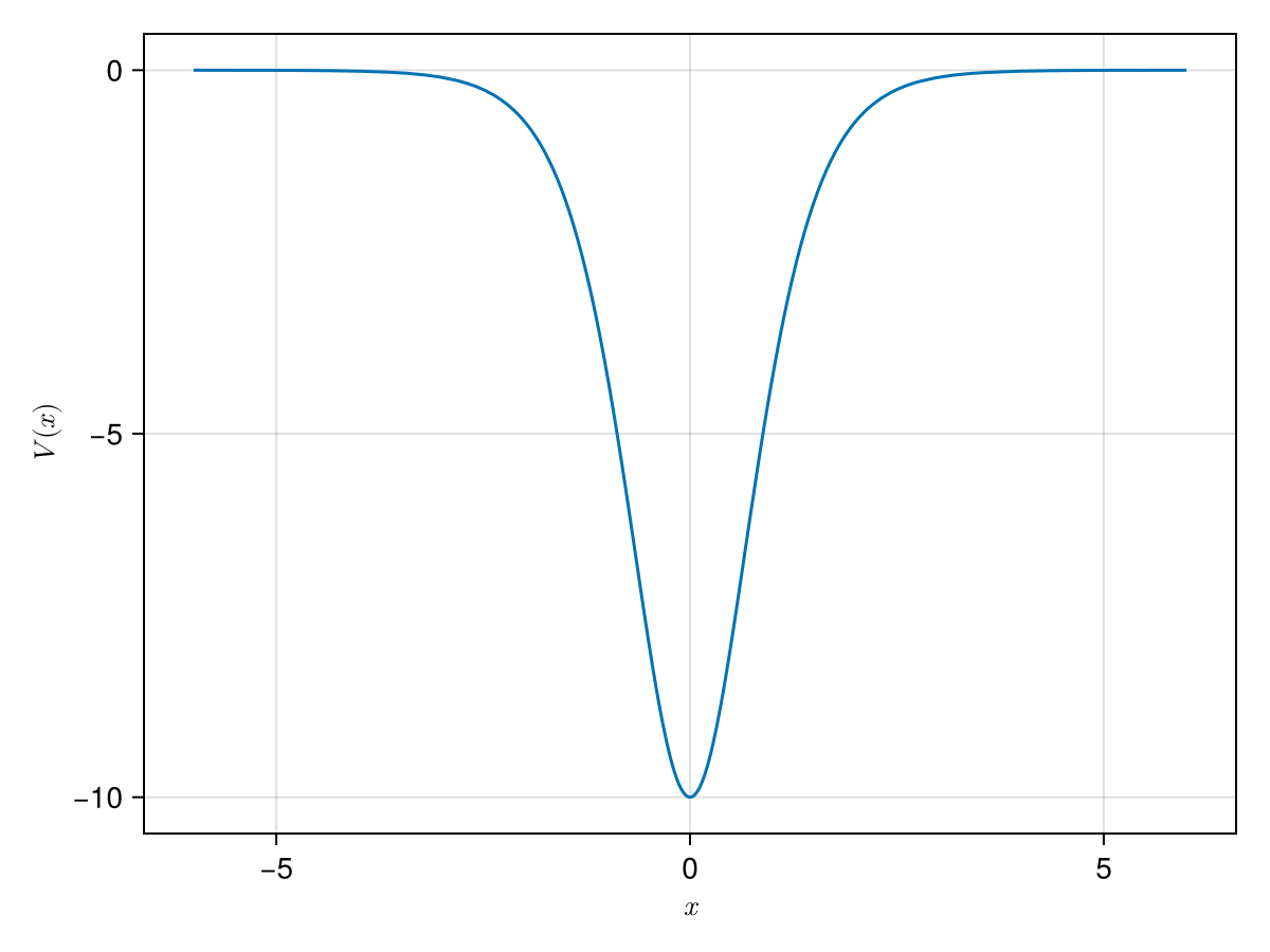

Wave functions:

using CairoMakie

# setting
f = Figure()
ax = Axis(f[1,1], xlabel=L"$x$", ylabel=L"$\psi(x)$")

# plot
w0 = lines!(ax, -3..3, x -> ψ(PT, x, n=0))
w1 = lines!(ax, -3..3, x -> ψ(PT, x, n=1))
w2 = lines!(ax, -3..3, x -> ψ(PT, x, n=2))
w3 = lines!(ax, -3..3, x -> ψ(PT, x, n=3))

# legend
axislegend(ax, [w0, w1, w2, w3], [L"n=0", L"n=1", L"n=2", L"n=3"], position=:lb)

f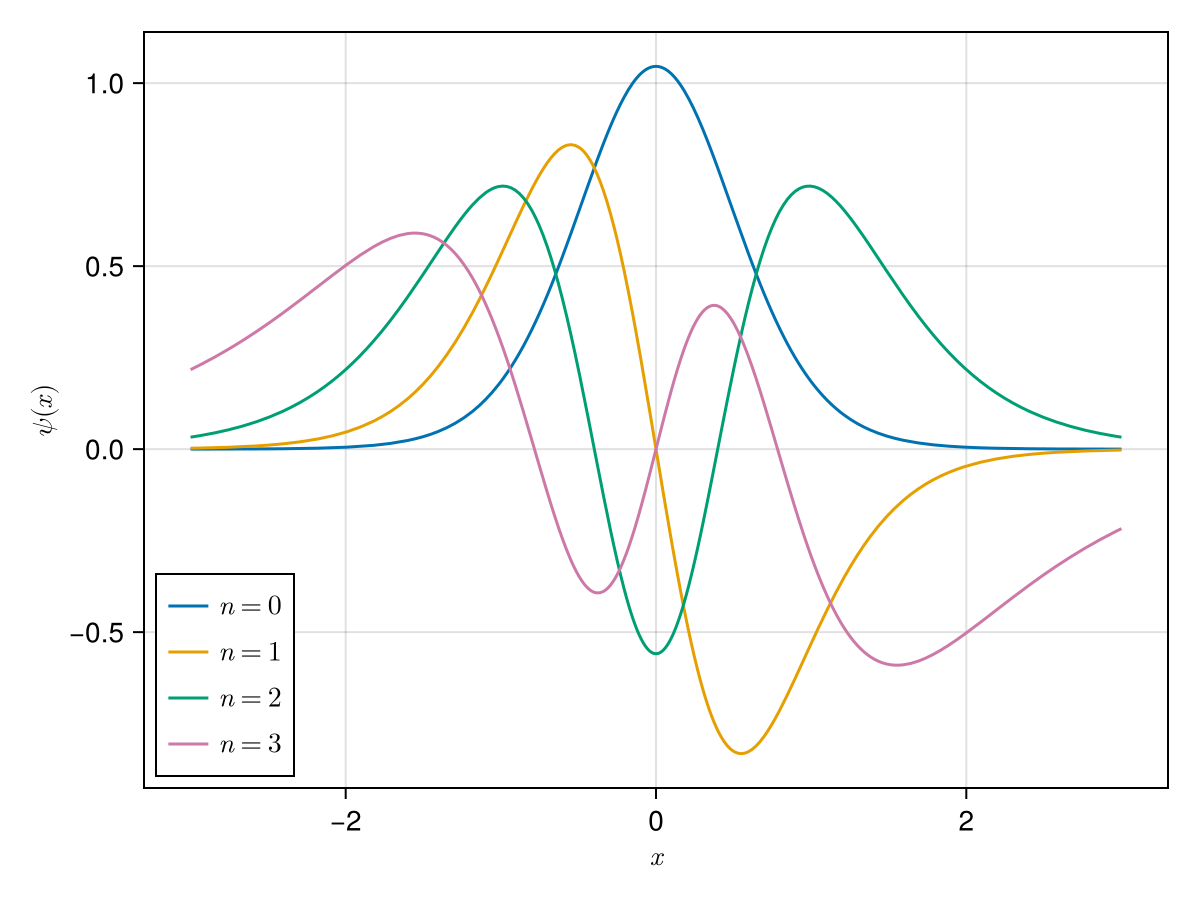

Potential energy curve, Energy levels, Wave functions:

using CairoMakie

# settings
f = Figure()
ax = Axis(f[1,1], xlabel=L"$x$", ylabel=L"$V(x),~E_n,~\psi_n(x) \times 5 + E_n$", aspect=1, limits=(-4,4,-10.5,1))
# hidespines!(ax)
# hidedecorations!(ax)

for n in 0:3
  # classical turning point
  xE = acosh(sqrt(PT.λ*(PT.λ+1)/abs(E(PT,n=n))/2))
  # energy
  hlines!(ax, E(PT, n=n), color=:black, linewidth=1, linestyle=:dash)
  lines!(ax, [-xE,xE], fill(E(PT,n=n),2), color=:black, linewidth=2)
  # wave function
  lines!(ax, -4..4, x -> E(PT,n=n) + ψ(PT,x,n=n), linewidth=2)
end

#potential
lines!(ax, -4..4, x -> V(PT,x), color=:black, linewidth=2)

f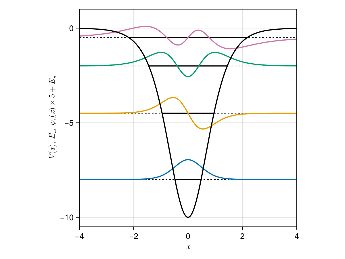

Testing

Unit testing and Integration testing were done using numerical integration (QuadGK.jl). The test script is here.

Associated Legendre Polynomials $P_n^m(x)$

\[ \begin{aligned} P_n^m(x) &= (-1)^m \left( 1-x^2 \right)^{m/2} \frac{\mathrm{d}^m}{\mathrm{d}x^m} P_n(x) \\ &= (-1)^m \left( 1-x^2 \right)^{m/2} \frac{\mathrm{d}^m}{\mathrm{d}x^m} \frac{1}{2^n n!} \frac{\mathrm{d}^n}{\mathrm{d}x ^n} \left[ \left( x^2-1 \right)^n \right] \\ &= \frac{(-1)^m}{2^n} (1-x^2)^{m/2} \sum_{j=0}^{\left\lfloor\frac{n-m}{2}\right\rfloor} (-1)^j \frac{(2n-2j)!}{j! (n-j)! (n-2j-m)!} x^{(n-2j-m)}. \end{aligned}\]

$n=0, m=0:$ ✔

\[\begin{aligned} P_{0}^{0}(x) = 1 &= 1 \\ &= 1 \end{aligned}\]

$n=1, m=0:$ ✔

\[\begin{aligned} P_{1}^{0}(x) = \frac{1}{2} \frac{\mathrm{d}}{\mathrm{d}x} \left( -1 + x^{2} \right) &= x \\ &= x \end{aligned}\]

$n=1, m=1:$ ✔

\[\begin{aligned} P_{1}^{1}(x) = - \left( 1 - x^{2} \right)^{\frac{1}{2}} \frac{\mathrm{d}}{\mathrm{d}x} \frac{1}{2} \frac{\mathrm{d}}{\mathrm{d}x} \left( -1 + x^{2} \right) &= - \left( 1 - x^{2} \right)^{\frac{1}{2}} \\ &= - \left( 1 - x^{2} \right)^{\frac{1}{2}} \end{aligned}\]

$n=2, m=0:$ ✔

\[\begin{aligned} P_{2}^{0}(x) = \frac{1}{8} \frac{\mathrm{d}}{\mathrm{d}x} \frac{\mathrm{d}}{\mathrm{d}x} \left( -1 + x^{2} \right)^{2} &= \frac{-1}{2} + \frac{3}{2} x^{2} \\ &= \frac{-1}{2} + \frac{3}{2} x^{2} \end{aligned}\]

$n=2, m=1:$ ✔

\[\begin{aligned} P_{2}^{1}(x) = - \left( 1 - x^{2} \right)^{\frac{1}{2}} \frac{\mathrm{d}}{\mathrm{d}x} \frac{1}{8} \frac{\mathrm{d}}{\mathrm{d}x} \frac{\mathrm{d}}{\mathrm{d}x} \left( -1 + x^{2} \right)^{2} &= - 3 \left( 1 - x^{2} \right)^{\frac{1}{2}} x \\ &= - 3 \left( 1 - x^{2} \right)^{\frac{1}{2}} x \end{aligned}\]

$n=2, m=2:$ ✔

\[\begin{aligned} P_{2}^{2}(x) = \left( 1 - x^{2} \right) \frac{\mathrm{d}}{\mathrm{d}x} \frac{\mathrm{d}}{\mathrm{d}x} \frac{1}{8} \frac{\mathrm{d}}{\mathrm{d}x} \frac{\mathrm{d}}{\mathrm{d}x} \left( -1 + x^{2} \right)^{2} &= 3 - 3 x^{2} \\ &= 3 - 3 x^{2} \end{aligned}\]

$n=3, m=0:$ ✔

\[\begin{aligned} P_{3}^{0}(x) = \frac{1}{48} \frac{\mathrm{d}}{\mathrm{d}x} \frac{\mathrm{d}}{\mathrm{d}x} \frac{\mathrm{d}}{\mathrm{d}x} \left( -1 + x^{2} \right)^{3} &= - \frac{3}{2} x + \frac{5}{2} x^{3} \\ &= - \frac{3}{2} x + \frac{5}{2} x^{3} \end{aligned}\]

$n=3, m=1:$ ✔

\[\begin{aligned} P_{3}^{1}(x) = - \left( 1 - x^{2} \right)^{\frac{1}{2}} \frac{\mathrm{d}}{\mathrm{d}x} \frac{1}{48} \frac{\mathrm{d}}{\mathrm{d}x} \frac{\mathrm{d}}{\mathrm{d}x} \frac{\mathrm{d}}{\mathrm{d}x} \left( -1 + x^{2} \right)^{3} &= \frac{3}{2} \left( 1 - x^{2} \right)^{\frac{1}{2}} - \frac{15}{2} x^{2} \left( 1 - x^{2} \right)^{\frac{1}{2}} \\ &= \frac{3}{2} \left( 1 - x^{2} \right)^{\frac{1}{2}} - \frac{15}{2} x^{2} \left( 1 - x^{2} \right)^{\frac{1}{2}} \end{aligned}\]

$n=3, m=2:$ ✔

\[\begin{aligned} P_{3}^{2}(x) = \left( 1 - x^{2} \right) \frac{\mathrm{d}}{\mathrm{d}x} \frac{\mathrm{d}}{\mathrm{d}x} \frac{1}{48} \frac{\mathrm{d}}{\mathrm{d}x} \frac{\mathrm{d}}{\mathrm{d}x} \frac{\mathrm{d}}{\mathrm{d}x} \left( -1 + x^{2} \right)^{3} &= 15 x - 15 x^{3} \\ &= 15 x - 15 x^{3} \end{aligned}\]

$n=3, m=3:$ ✔

\[\begin{aligned} P_{3}^{3}(x) = - \left( 1 - x^{2} \right)^{\frac{3}{2}} \frac{\mathrm{d}}{\mathrm{d}x} \frac{\mathrm{d}}{\mathrm{d}x} \frac{\mathrm{d}}{\mathrm{d}x} \frac{1}{48} \frac{\mathrm{d}}{\mathrm{d}x} \frac{\mathrm{d}}{\mathrm{d}x} \frac{\mathrm{d}}{\mathrm{d}x} \left( -1 + x^{2} \right)^{3} &= - 15 \left( 1 - x^{2} \right)^{\frac{3}{2}} \\ &= - 15 \left( 1 - x^{2} \right)^{\frac{3}{2}} \end{aligned}\]

$n=4, m=0:$ ✔

\[\begin{aligned} P_{4}^{0}(x) = \frac{1}{384} \frac{\mathrm{d}}{\mathrm{d}x} \frac{\mathrm{d}}{\mathrm{d}x} \frac{\mathrm{d}}{\mathrm{d}x} \frac{\mathrm{d}}{\mathrm{d}x} \left( -1 + x^{2} \right)^{4} &= \frac{3}{8} - \frac{15}{4} x^{2} + \frac{35}{8} x^{4} \\ &= \frac{3}{8} - \frac{15}{4} x^{2} + \frac{35}{8} x^{4} \end{aligned}\]

$n=4, m=1:$ ✔

\[\begin{aligned} P_{4}^{1}(x) = - \left( 1 - x^{2} \right)^{\frac{1}{2}} \frac{\mathrm{d}}{\mathrm{d}x} \frac{1}{384} \frac{\mathrm{d}}{\mathrm{d}x} \frac{\mathrm{d}}{\mathrm{d}x} \frac{\mathrm{d}}{\mathrm{d}x} \frac{\mathrm{d}}{\mathrm{d}x} \left( -1 + x^{2} \right)^{4} &= \frac{15}{2} \left( 1 - x^{2} \right)^{\frac{1}{2}} x - \frac{35}{2} x^{3} \left( 1 - x^{2} \right)^{\frac{1}{2}} \\ &= \frac{15}{2} \left( 1 - x^{2} \right)^{\frac{1}{2}} x - \frac{35}{2} x^{3} \left( 1 - x^{2} \right)^{\frac{1}{2}} \end{aligned}\]

$n=4, m=2:$ ✔

\[\begin{aligned} P_{4}^{2}(x) = \left( 1 - x^{2} \right) \frac{\mathrm{d}}{\mathrm{d}x} \frac{\mathrm{d}}{\mathrm{d}x} \frac{1}{384} \frac{\mathrm{d}}{\mathrm{d}x} \frac{\mathrm{d}}{\mathrm{d}x} \frac{\mathrm{d}}{\mathrm{d}x} \frac{\mathrm{d}}{\mathrm{d}x} \left( -1 + x^{2} \right)^{4} &= \frac{-15}{2} + 60 x^{2} - \frac{105}{2} x^{4} \\ &= \frac{-15}{2} + 60 x^{2} - \frac{105}{2} x^{4} \end{aligned}\]

$n=4, m=3:$ ✔

\[\begin{aligned} P_{4}^{3}(x) = - \left( 1 - x^{2} \right)^{\frac{3}{2}} \frac{\mathrm{d}}{\mathrm{d}x} \frac{\mathrm{d}}{\mathrm{d}x} \frac{\mathrm{d}}{\mathrm{d}x} \frac{1}{384} \frac{\mathrm{d}}{\mathrm{d}x} \frac{\mathrm{d}}{\mathrm{d}x} \frac{\mathrm{d}}{\mathrm{d}x} \frac{\mathrm{d}}{\mathrm{d}x} \left( -1 + x^{2} \right)^{4} &= - 105 \left( 1 - x^{2} \right)^{\frac{3}{2}} x \\ &= - 105 \left( 1 - x^{2} \right)^{\frac{3}{2}} x \end{aligned}\]

$n=4, m=4:$ ✔

\[\begin{aligned} P_{4}^{4}(x) = \left( 1 - x^{2} \right)^{2} \frac{\mathrm{d}}{\mathrm{d}x} \frac{\mathrm{d}}{\mathrm{d}x} \frac{\mathrm{d}}{\mathrm{d}x} \frac{\mathrm{d}}{\mathrm{d}x} \frac{1}{384} \frac{\mathrm{d}}{\mathrm{d}x} \frac{\mathrm{d}}{\mathrm{d}x} \frac{\mathrm{d}}{\mathrm{d}x} \frac{\mathrm{d}}{\mathrm{d}x} \left( -1 + x^{2} \right)^{4} &= 105 \left( 1 - x^{2} \right)^{2} \\ &= 105 \left( 1 - x^{2} \right)^{2} \end{aligned}\]

Normalization & Orthogonality of $\psi_n(x)$

\[\int \psi_i^\ast(x) \psi_j(x) \mathrm{d}x = \delta_{ij}\]

 i |  j |        analytical |         numerical 
-- | -- | ----------------- | ----------------- 
 0 |  0 |    1.000000000000 |    1.000000000000 ✔
 0 |  1 |    0.000000000000 |   -0.000000000000 ✔
 0 |  2 |    0.000000000000 |    0.000000000000 ✔
 0 |  3 |    0.000000000000 |    0.000000000000 ✔
 0 |  4 |    0.000000000000 |   -0.000000000000 ✔
 0 |  5 |    0.000000000000 |   -0.000000000000 ✔
 0 |  6 |    0.000000000000 |    0.000000000000 ✔
 0 |  7 |    0.000000000000 |   -0.000000000000 ✔
 0 |  8 |    0.000000000000 |   -0.000000000000 ✔
 0 |  9 |    0.000000000000 |    0.000000000000 ✔
 1 |  0 |    0.000000000000 |   -0.000000000000 ✔
 1 |  1 |    1.000000000000 |    1.000000000000 ✔
 1 |  2 |    0.000000000000 |   -0.000000000000 ✔
 1 |  3 |    0.000000000000 |    0.000000000000 ✔
 1 |  4 |    0.000000000000 |    0.000000000000 ✔
 1 |  5 |    0.000000000000 |   -0.000000000000 ✔
 1 |  6 |    0.000000000000 |   -0.000000000000 ✔
 1 |  7 |    0.000000000000 |    0.000000000000 ✔
 1 |  8 |    0.000000000000 |   -0.000000000000 ✔
 1 |  9 |    0.000000000000 |    0.000000000000 ✔
 2 |  0 |    0.000000000000 |    0.000000000000 ✔
 2 |  1 |    0.000000000000 |   -0.000000000000 ✔
 2 |  2 |    1.000000000000 |    1.000000000000 ✔
 2 |  3 |    0.000000000000 |    0.000000000000 ✔
 2 |  4 |    0.000000000000 |    0.000000000000 ✔
 2 |  5 |    0.000000000000 |   -0.000000000000 ✔
 2 |  6 |    0.000000000000 |   -0.000000000000 ✔
 2 |  7 |    0.000000000000 |    0.000000000000 ✔
 2 |  8 |    0.000000000000 |   -0.000000000000 ✔
 2 |  9 |    0.000000000000 |   -0.000000000000 ✔
 3 |  0 |    0.000000000000 |    0.000000000000 ✔
 3 |  1 |    0.000000000000 |    0.000000000000 ✔
 3 |  2 |    0.000000000000 |    0.000000000000 ✔
 3 |  3 |    1.000000000000 |    1.000000000000 ✔
 3 |  4 |    0.000000000000 |    0.000000000000 ✔
 3 |  5 |    0.000000000000 |    0.000000000000 ✔
 3 |  6 |    0.000000000000 |   -0.000000000000 ✔
 3 |  7 |    0.000000000000 |    0.000000000000 ✔
 3 |  8 |    0.000000000000 |    0.000000000000 ✔
 3 |  9 |    0.000000000000 |    0.000000000000 ✔
 4 |  0 |    0.000000000000 |   -0.000000000000 ✔
 4 |  1 |    0.000000000000 |    0.000000000000 ✔
 4 |  2 |    0.000000000000 |    0.000000000000 ✔
 4 |  3 |    0.000000000000 |    0.000000000000 ✔
 4 |  4 |    1.000000000000 |    0.999999999999 ✔
 4 |  5 |    0.000000000000 |   -0.000000000000 ✔
 4 |  6 |    0.000000000000 |    0.000000000000 ✔
 4 |  7 |    0.000000000000 |    0.000000000000 ✔
 4 |  8 |    0.000000000000 |    0.000000000000 ✔
 4 |  9 |    0.000000000000 |    0.000000000000 ✔
 5 |  0 |    0.000000000000 |   -0.000000000000 ✔
 5 |  1 |    0.000000000000 |   -0.000000000000 ✔
 5 |  2 |    0.000000000000 |   -0.000000000000 ✔
 5 |  3 |    0.000000000000 |    0.000000000000 ✔
 5 |  4 |    0.000000000000 |   -0.000000000000 ✔
 5 |  5 |    1.000000000000 |    1.000000000000 ✔
 5 |  6 |    0.000000000000 |   -0.000000000000 ✔
 5 |  7 |    0.000000000000 |   -0.000000000000 ✔
 5 |  8 |    0.000000000000 |    0.000000000000 ✔
 5 |  9 |    0.000000000000 |    0.000000000000 ✔
 6 |  0 |    0.000000000000 |    0.000000000000 ✔
 6 |  1 |    0.000000000000 |   -0.000000000000 ✔
 6 |  2 |    0.000000000000 |   -0.000000000000 ✔
 6 |  3 |    0.000000000000 |   -0.000000000000 ✔
 6 |  4 |    0.000000000000 |    0.000000000000 ✔
 6 |  5 |    0.000000000000 |   -0.000000000000 ✔
 6 |  6 |    1.000000000000 |    1.000000000000 ✔
 6 |  7 |    0.000000000000 |   -0.000000000000 ✔
 6 |  8 |    0.000000000000 |    0.000000000000 ✔
 6 |  9 |    0.000000000000 |   -0.000000000000 ✔
 7 |  0 |    0.000000000000 |   -0.000000000000 ✔
 7 |  1 |    0.000000000000 |    0.000000000000 ✔
 7 |  2 |    0.000000000000 |    0.000000000000 ✔
 7 |  3 |    0.000000000000 |    0.000000000000 ✔
 7 |  4 |    0.000000000000 |    0.000000000000 ✔
 7 |  5 |    0.000000000000 |   -0.000000000000 ✔
 7 |  6 |    0.000000000000 |   -0.000000000000 ✔
 7 |  7 |    1.000000000000 |    1.000000000000 ✔
 7 |  8 |    0.000000000000 |    0.000000000000 ✔
 7 |  9 |    0.000000000000 |    0.000000000000 ✔
 8 |  0 |    0.000000000000 |   -0.000000000000 ✔
 8 |  1 |    0.000000000000 |   -0.000000000000 ✔
 8 |  2 |    0.000000000000 |   -0.000000000000 ✔
 8 |  3 |    0.000000000000 |    0.000000000000 ✔
 8 |  4 |    0.000000000000 |    0.000000000000 ✔
 8 |  5 |    0.000000000000 |    0.000000000000 ✔
 8 |  6 |    0.000000000000 |    0.000000000000 ✔
 8 |  7 |    0.000000000000 |    0.000000000000 ✔
 8 |  8 |    1.000000000000 |    1.000000000000 ✔
 8 |  9 |    0.000000000000 |    0.000000000000 ✔
 9 |  0 |    0.000000000000 |    0.000000000000 ✔
 9 |  1 |    0.000000000000 |    0.000000000000 ✔
 9 |  2 |    0.000000000000 |   -0.000000000000 ✔
 9 |  3 |    0.000000000000 |    0.000000000000 ✔
 9 |  4 |    0.000000000000 |    0.000000000000 ✔
 9 |  5 |    0.000000000000 |    0.000000000000 ✔
 9 |  6 |    0.000000000000 |   -0.000000000000 ✔
 9 |  7 |    0.000000000000 |    0.000000000000 ✔
 9 |  8 |    0.000000000000 |    0.000000000000 ✔
 9 |  9 |    1.000000000000 |    1.000000000000 ✔

Eigen Values

\[ \begin{aligned} E_n &= \int \psi^\ast_n(x) \hat{H} \psi_n(x) \mathrm{d}x \\ &= \int \psi^\ast_n(x) \left[ \hat{V} + \hat{T} \right] \psi(x) \mathrm{d}x \\ &= \int \psi^\ast_n(x) \left[ V(x) - \frac{\hbar^2}{2m} \frac{\mathrm{d}^{2}}{\mathrm{d} x^{2}} \right] \psi(x) \mathrm{d}x \\ &\simeq \int \psi^\ast_n(x) \left[ V(x)\psi(x) -\frac{\hbar^2}{2m} \frac{\psi(x+\Delta x) - 2\psi(x) + \psi(x-\Delta x)}{\Delta x^{2}} \right] \mathrm{d}x. \end{aligned}\]

Where, the difference formula for the 2nd-order derivative:

\[\begin{aligned} % 2\psi(x) % + \frac{\mathrm{d}^{2} \psi(x)}{\mathrm{d} x^{2}} \Delta x^{2} % + O\left(\Delta x^{4}\right) % &= % \psi(x+\Delta x) % + \psi(x-\Delta x) % \\ % \frac{\mathrm{d}^{2} \psi(x)}{\mathrm{d} x^{2}} \Delta x^{2} % &= % \psi(x+\Delta x) % - 2\psi(x) % + \psi(x-\Delta x) % - O\left(\Delta x^{4}\right) % \\ % \frac{\mathrm{d}^{2} \psi(x)}{\mathrm{d} x^{2}} % &= % \frac{\psi(x+\Delta x) - 2\psi(x) + \psi(x-\Delta x)}{\Delta x^{2}} % - \frac{O\left(\Delta x^{4}\right)}{\Delta x^{2}} % \\ \frac{\mathrm{d}^{2} \psi(x)}{\mathrm{d} x^{2}} &= \frac{\psi(x+\Delta x) - 2\psi(x) + \psi(x-\Delta x)}{\Delta x^{2}} + O\left(\Delta x^{2}\right) \end{aligned}\]

are given by the sum of 2 Taylor series:

\[\begin{aligned} \psi(x+\Delta x) &= \psi(x) + \frac{\mathrm{d} \psi(x)}{\mathrm{d} x} \Delta x + \frac{1}{2!} \frac{\mathrm{d}^{2} \psi(x)}{\mathrm{d} x^{2}} \Delta x^{2} + \frac{1}{3!} \frac{\mathrm{d}^{3} \psi(x)}{\mathrm{d} x^{3}} \Delta x^{3} + O\left(\Delta x^{4}\right), \\ \psi(x-\Delta x) &= \psi(x) - \frac{\mathrm{d} \psi(x)}{\mathrm{d} x} \Delta x + \frac{1}{2!} \frac{\mathrm{d}^{2} \psi(x)}{\mathrm{d} x^{2}} \Delta x^{2} - \frac{1}{3!} \frac{\mathrm{d}^{3} \psi(x)}{\mathrm{d} x^{3}} \Delta x^{3} + O\left(\Delta x^{4}\right). \end{aligned}\]

  λ |  n |        analytical |         numerical 
--- | -- | ----------------- | ----------------- 
1.0 |  0 |   -0.500000000000 |   -0.500000019503 ✔
2.0 |  0 |   -2.000000000000 |   -2.000000095274 ✔
2.0 |  1 |   -0.500000000000 |   -0.500000184608 ✔
3.0 |  0 |   -4.500000000000 |   -4.500000232181 ✔
3.0 |  1 |   -2.000000000000 |   -2.000000666754 ✔
3.0 |  2 |   -0.500000000000 |   -0.500000670248 ✔
5.0 |  0 |  -12.500000000000 |  -12.500000692040 ✔
5.0 |  1 |   -8.000000000000 |   -8.000002554891 ✔
5.0 |  2 |   -4.500000000000 |   -4.500004389011 ✔
5.0 |  3 |   -2.000000000000 |   -2.000004722624 ✔
5.0 |  4 |   -0.500000000000 |   -0.500003083668 ✔

References

- [7] G. Pöschl, E. Teller, Zeitschrift für Physik, 83 (3–4), 143 (1933), (https://doi.org/10.1007%2FBF01331132). More general definitions are given as (2a), (2b) or (11)
- [8] S. Flügge, Practical Quantum Mechanics (Springer Berlin Heidelberg, 1999), (https://doi.org/10.1007/978-3-642-61995-3) p.94 Problem 39. Potential hole of modified Poschl-Teller type
Potential
Maximum Quantum Number